偏差|泰勒_滤波跟踪基于matlab北方苍鹰和粒子群算法优化粒子滤波器目标滤波跟踪含Matlab源码2260期

篇首语：本文由编程笔记#小编为大家整理，主要介绍了滤波跟踪基于matlab北方苍鹰和粒子群算法优化粒子滤波器目标滤波跟踪含Matlab源码 2260期相关的知识，希望对你有一定的参考价值。

⛄一、EKF算法简介

扩展卡尔曼滤波是利用泰勒级数展开方法将非线性滤波问题转化成近似的线性滤波问题,利用线性滤波的理论求解非线性滤波问题的次优滤波算法。其系统的状态方程和量测方程分别如式(1)、式(2)所示:

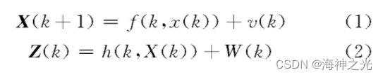
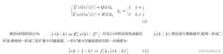
式中,X(k)为n维的随机状态向量序列,Z(k)为n维的随机量测向量序列,f(k,x(k))为空气阻力,v(k)、w(k)为零均值的正态(高斯)白噪声序列,其方差分别满足:

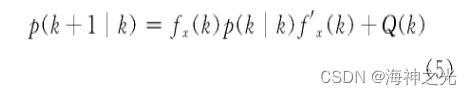
协方差的一步预测为:

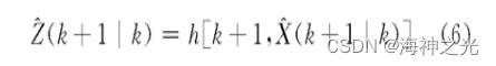
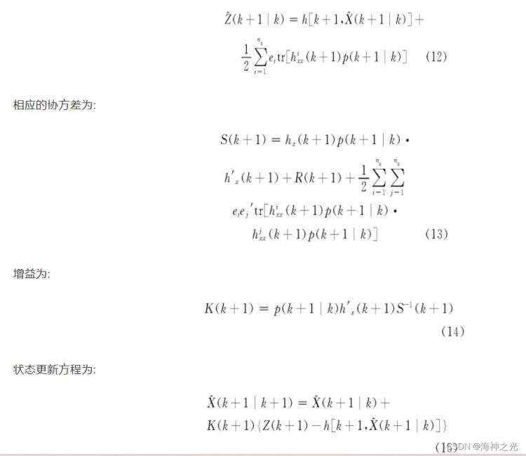
量测预测值为:

相应的协方差为:

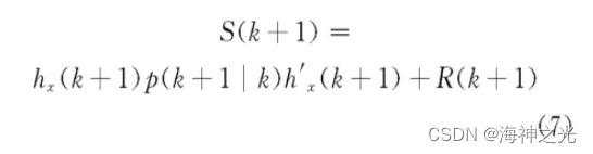
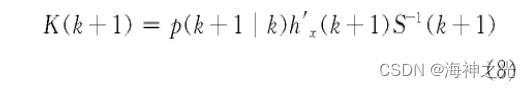
增益为:

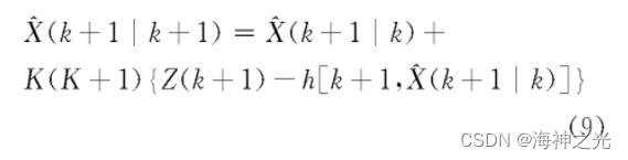
状态更新方程为:

协方差更新方程为:

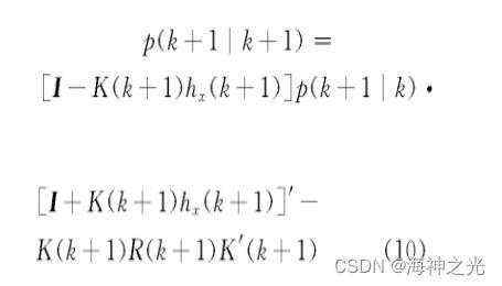
式中,I为与协方差同维的单位矩阵。

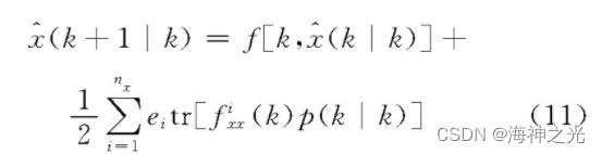
二阶扩展卡尔曼滤波的泰勒展开保留到二阶项,其状态的一步预测为:

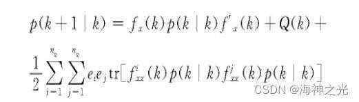
协方差的一步预测为:

量测预测值为:

协方差更新方程为:

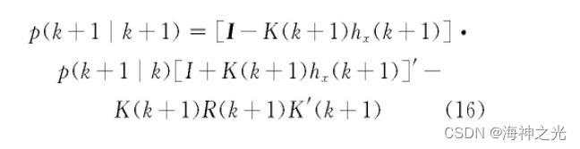
式中,I为与协方差同维的单位矩阵。

⛄二、部分源代码

function main
rand(‘seed’,3);
randn(‘seed’,6);
T&＃61;50;
R&＃61;1e-5;
P&＃61;1;%观测误差
Q&＃61;0.01;%预测误差
X&＃61;zeros(1,T);
Z&＃61;zeros(1,T);
X(1)&＃61;1;
Z(1)&＃61;1;

%基本粒子滤波设置
N&＃61;50;
Xpf&＃61;zeros(1,T);
Xpfset&＃61;ones(T,N);
Tpf&＃61;zeros(1,T);
%
% %PSOPF
Xpsopf&＃61;zeros(1,T);
Xpsopfset&＃61;ones(T,N);
Tpsopf&＃61;zeros(1,T);

%NGOPF
Xngopf&＃61;zeros(1,T);
Xngopfset&＃61;ones(T,N);
Tngopf&＃61;zeros(1,T);

%模拟运行
for t&＃61;2:T
X(t)&＃61;feval(‘ffun’,X(t-1),t,Q);
Z(t)&＃61;feval(‘hfun’,X(t),P);

% %PF
tic
[Xpf(t),Xpfset(t,:)]&＃61;pf(Xpfset(t-1,:),Z(t),N,t,R,P,Q);
Tpf(t)&＃61;toc;

% %PSOPF
tic
[Xpsopf(t),Xpsopfset(t,:)]&＃61;pso_pf(Xpsopfset(t-1,:),Z(t),N,t,R,P,Q);
Tpsopf(t)&＃61;toc;

%NGOPF
tic
[Xngopf(t),Xngopfset(t,:)]&＃61;ngo_pf(Xngopfset(t-1,:),Z(t),N,t,R,P,Q);
%[Xngopf(t),Xngopfset(t,:)]&＃61;ngo_pf1(Xngopfset(t-1,:),Z(t),N,t,R,P,Q);
Tngopf(t)&＃61;toc;

end;

ErrorPf&＃61;abs(Xpf-X);
ErrorPsoPf&＃61;abs(Xpsopf-X);
ErrorNgoPf&＃61;abs(Xngopf-X);

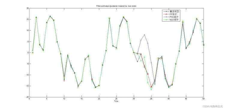
%picture
figure
hold on;
box on;
p1&＃61;plot(1:T,X,‘-k.’,‘LineWidth’,1);
p2&＃61;plot(1:T,Xpf,‘-ro’,‘LineWidth’,1);
p3&＃61;plot(1:T,Xpsopf,‘-bx’,‘LineWidth’,1);
p4&＃61;plot(1:T,Xngopf,‘-gd’,‘LineWidth’,1);
legend([p1,p2,p3,p4],‘真实状态’,‘PF估计’,‘PSO估计’,‘NGO估计’)
xlabel(‘Time’,‘fontsize’,10)
title(‘Filter estmates (posterior means) vs. ture state’,‘fontsize’,10)

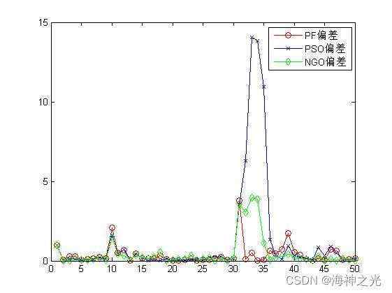
%偏差比较
figure
hold on;
box on;
p1&＃61;plot(1:T,ErrorPf,‘-ro’,‘LineWidth’,1);
p2&＃61;plot(1:T,ErrorPsoPf,‘-bx’,‘LineWidth’,1);
p3&＃61;plot(1:T,ErrorNgoPf,‘-gd’,‘LineWidth’,1);
legend([p1,p2,p3],‘PF偏差’,‘PSO偏差’,‘NGO偏差’)

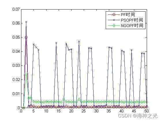
%算法Time比较图
figure
hold on;
box on;
p1&＃61;plot(1:T,Tpf,‘-ro’,‘LineWidth’,1);
p2&＃61;plot(1:T,Tpsopf,‘-bx’,‘LineWidth’,1);
p3&＃61;plot(1:T,Tngopf,‘-gd’,‘LineWidth’,1);
legend([p1,p2,p3],‘PF时间’,‘PSOPF时间’,‘NGOPF时间’)

%

⛄三、运行结果

⛄四、matlab版本及参考文献

1 matlab版本
2014a

2 参考文献
[1]宁倩慧,张艳兵,刘莉,陆真,郭冰陶.扩展卡尔曼滤波的目标跟踪优化算法[J].探测与控制学报. 2016,38(01)

3 备注
简介此部分摘自互联网&＃xff0c;仅供参考&＃xff0c;若侵权&＃xff0c;联系删除